Decoding X-ray Hand Bones | Semantic Segmentation

1. Introduction

Bone Segmentation is one of the most important applications in Artificial Intelligence, using deep learning technologies to find and segment individual bone.

Thanks to boostcamp AI Tech, our team can work on a project to segment and analyze hand bones using semantic segmentation models for a medical image dataset, generally hard to obtain.

As a team leader on this project, I contributed to managing our project schedule, creating a visualization tool to analyze dataset or experiment results, conducting model experiment based on relevant libraries, and carrying out ensemble to improve the final result of our models.

2. Exploratory Data Analysis (EDA)

2.1. Visualization Tool

A visualization tool is introduced using Streamlit, an open-source framework for AI/ML engineers. To analyze the image data properly, we needed features as follows.

• Compare (image vs label, image vs model result, model result vs label)
• Toggle the visibility of labels by class
• Upload experiment result (in csv format)

Considering all the requirements above, I made web demo for data(images & labels) visualization as below. You can find the code here.

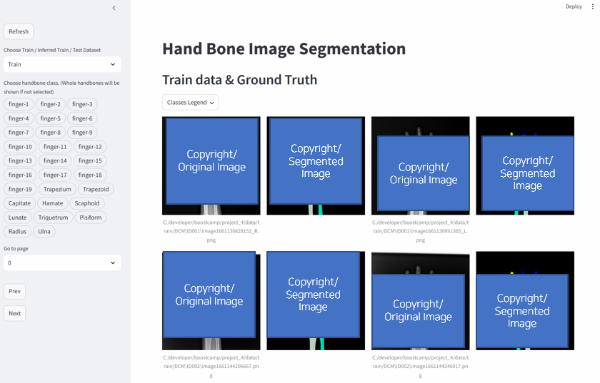Visualization Web Demo

2.2. What we found

Through our web visualizer, we found a few things to consider in this project. First, the pixels on the wrist bone are overlapped compared to the finger bones. It would be effective to choose a model that works for medical images. Next, some bones such as fingertip or wrist are too small to identify with naked eyes. Enlarging the image could be a solution. Also, small number of data is also one of the limitations to improve the performance of our model.

3. Model Experiments

3.1. Segmentation models

Segmentation has already been developed as a relatively traditional deep learning technology in AI, which changes so quickly. Fortunately, there is a library, called Segmentation Models, which supports various segmentation models and encoders. To conduct experiments quickly, we adopted this library. The interface for model application looks like as follows.

import segmentation_models_pytorch as smp


class SmpModel:
    def __init__(self, model_config, num_classes):
        self.arch = model_config['arch']
        self.encoder_name = model_config['encoder_name']
        self.encoder_weights = model_config['encoder_weights']
        self.in_channels = model_config['in_channels']
        self.num_classes = num_classes

    def get_model(self):
        self.model = smp.create_model(
            arch = self.arch,
            encoder_name = self.encoder_name,
            encoder_weights = self.encoder_weights,
            in_channels = self.in_channels,
            classes = self.num_classes,
        )
        
        return self.model 

Considering the characteristics of our dataset, I experimented with medical-originated models (UNet, MANet) or the latest models (UPerNet, SegFormer).

• UNet Series

Model	Backbone	Dice
UNet	ResNet50	0.9474
UNet++	ResNet50	0.9538
UNEt++	ResNet101	0.9517
UNEt++	Efficientnet-b5	0.9511
UNEt++	GerNet-L	0.9513

• MANet : Due to limited time, the training was executed with smaller image size(512 ➡️ 256) and less epochs (100 ➡️ 50)

Model	Backbone	Dice
UNet++	ResNet50	0.9101
MANet	ResNet50	0.8989
MANet	Res2Net50_26w_4s	0.8957
MANet	ResNest50d_4s2x40d	0.9026

• UPerNet

Model	Backbone	Dice
UperNet	ResNet101	0.9479
UperNet	swin transformer	0.9501

• SegFormer

Model	Backbone	Dice
SegFormer	mit-b0	0.9610

3.2. Augmentation

Furthermore, we performed off-line augmentation by cropping and enlarging small bones or wrist in order to solve small bone and overlapping problems.

• Size

As the below table shows, there was a significant performance improvement when the size increased. However, it was impossible to enlarge image size over 1024 due to memory limitations.

Image Size	Dice
256 x 256	0.8431
512 x 512	0.8575
1024 x 1024	0.9644

• Off-line augmentation

Through cropping wrist or/and fingertip images, we added more images into our dataset. The result shows that the performance was improved, which seems to be due to 1) an increase in the amount of data itself, 2) additional learning for the part that lacked training.

Class	Original	Wrist	Fingertip	Wrist + Fingertip
Lunate	0.9103	0.9366	0.9340	0.9316
Trapezoid	0.8705	0.8951	0.8917	0.9005
Pisiform	0.8232	0.8750	0.8689	0.8864
Trapezium	0.9110	0.9221	0.9082	0.9178
finger-16	0.8564	0.9060	0.9054	0.9002

4. Ensemble

In data science, ensemble learning is a technique that combines multiple models to make more accurate prediction. Hard voting-based ensemble was introduced to improve our model performance. Combining the prediction results of several models for each class pixels, it is reflected in the final result when vote result exceed threshold. The way how I coded is as follows.

import os
import numpy as np
import pandas as pd 
from tqdm import tqdm

def decode_rle_to_mask(rle, height, width):
    s = rle.split()
    starts, lengths = [np.asarray(x, dtype=int) for x in (s[0:][::2], s[1:][::2])]
    starts -= 1
    ends = starts + lengths
    img = np.zeros(height * width, dtype=np.uint8)
    
    for lo, hi in zip(starts, ends):
        img[lo:hi] = 1
    
    return img.reshape(height, width)

def encode_mask_to_rle(mask):
    pixels = mask.flatten()
    pixels = np.concatenate([[0], pixels, [0]])
    runs = np.where(pixels[1:] != pixels[:-1])[0] + 1
    runs[1::2] -= runs[::2]

    return ' '.join(str(x) for x in runs)

def csv_ensemble(csv_paths, save_dir, threshold): 

    csv_data = []
    for path in csv_paths:
        data = pd.read_csv(path)
        csv_data.append(data)

    file_num = len(csv_data)
    filename_and_class = []
    rles = []

    print(f"Model Number : {file_num}, threshold: {threshold}")  

    pivot_df = csv_data[0]

    for _, row  in tqdm(pivot_df.iterrows(), total=pivot_df.shape[0]):
        img = row['image_name']
        cls = row['class']
        model_rles = []

        for data in csv_data:
            rle_value = data[(data['image_name'] == img) & (data['class'] == cls)]['rle'].values
            if len(rle_value) == 0 or pd.isna(rle_value[0]): 
                print(f"No RLE Data : Image {img}, Class {cls}")
                model_rles.append(np.zeros((2048, 2048), dtype=np.uint8))  
                continue
            model_rles.append(decode_rle_to_mask(str(rle_value[0]), 2048, 2048))
     
        image = np.zeros((2048,2048))

        for model in model_rles:
            image += model
        
        image[image <= threshold] = 0
        image[image > threshold] = 1

        result_image = image

        rles.append(encode_mask_to_rle(result_image))
        filename_and_class.append(f"{cls}_{img}")

    classes, filename = zip(*[x.split("_") for x in filename_and_class])
    image_name = [os.path.basename(f) for f in filename]

    df = pd.DataFrame({
        "image_name": image_name,
        "class": classes,
        "rle": rles,
    })

    df.to_csv(save_dir, index=False)

5. Conclusion

5.1. Result

Based on the experiment results, we concluded and trained our final models for 100 epochs.

• Unet++ : Backbone(ResNet50), Image Size(1024)
• DeepLabV3 : Backbone(EfficientNet-b8), Image Size(1024)
• UperNet : Backbone(Swin Transformer), Image Size(1536)
• SegFormer : Backbone(mit-b0), Image Size(1024)

With the results, we could derive the best performance compared to the baseline. (3.4%🔺)

Model	Threshold	Dice
Ensemble (w/o Best)	1	0.9676
Ensemble (w/o Best)	2	0.9689
Ensemble (w/ Best)	1	0.9696

5.2. Copyright and Code

This project is a part of a project held at boostcamp AI Tech, managed by NAVER Connect Foundation. The dataset is only used for boostcamp education and not allowed to take outside, so this post includes very limited image. Furthermore, it is available to find more detailed code for this project in my GitHub.